For simple explicit constructions and examples the analytic techniques behind the theory presented above will be an essential obstruction. The theory may be reduced to C¹-curves which are piecewise C², and then there is a gateway for considering curves composed of pieces of circles with C¹-matchings for these pieces. Here everything can be reduced to the consideration of a finite set of data given by the finte number of circles in space. But the whole theory even can be broken down to the level of spatial polygons, and this opens a wide field for nice constructions which everybody can pursue on his own. Here just this concept should be presented in analogy to the preceding section, leaving explicit constructions to the reader.

Two simply closed polygons in space are called parallel, if there is a bijection between their vertices, mapping consecutive vertices to consecutive ones again, such that the angle-bisecting planes at corresponding vertices coincide. (It should be noted that this is more restrictive, than assuming that corresponding line segments are parallel.) A system of normal vectors to the edges of a polygon is called a parallel field of normals, if every two vectors belonging to edges with a common vertex are symmetric with respect to the reflection at the angle-bisecting plane of the polygon at this vertex. Then parallel polygons are related by a parallel normal vector field (of constant length) again. A self-parallelism or tangential symmetry is just a combinatorial automorphism of the combinatorial structure behind the polygon, such that the original and the relabelled polygon are parallel.

Furthermore, if a closed polygon possesses a non-trivial self-parallelism, then its total normal twist (which is defined in obvious analogy to the smooth case) vanishes mod 2p. We have the same kind of classification for tangentially symmetric polygons like in the smooth case:
    i) Assume that the polygon P in E³ admits a parallel section in the normal bundle of its k-fold covering, then the obvious construction of a parallel at suitable distance has Z_k as its group of self-parallelisms.
    ii) Viceversa, every polygon possessing more than one self-parallelism can be obtained by the preceding construction from a suitable central polygon.

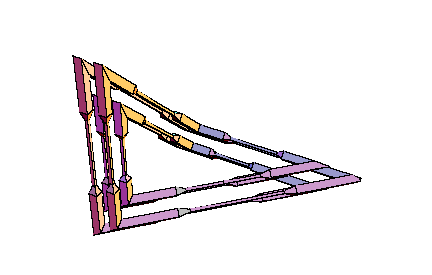
Details for these considerations can be found in [W5]. Very explicit calculations in the case of spatial quadrilaterals as center polygons have been obtained in [W6]. Everything can be reduced to the framework of elementary Euclidean geometry in 3-space. Examples of self-parallel polygons, which are not restricted to a plane, start with 8 vertices at least. Those with 8 vertices bound a PL-Moebius strip, and the central quadrilateral has to satisfy very special constraints for its angles and side lengths. Constructions with pentagons as central polygons are easier to visualize. They provide very simple families of imbedded PL-Moebius strips having a bounding polygon with 10 vertices, such that the strip may be composed from planar pieces of constant breadth. This is the case of symmetry group Z₂.

For symmetry group Z₄ and a center quadrilateral we receive recipes for composing four bars with the same square as their profile, such that the result will be a skew frame and such that the edges resulting from the bars form one connected closed polygon (with 16 vertices). The common picture frames have a planar rectangle as their basis, and the edges coming from the bars decompose into four rectangles of different sizes. It is easy to produce wooden models for these skew frames also by cutting the bars into pieces of appropriate lengths, such that planes for the sawing have the right angle with respect to the center line of the bar. Comparing this model with other models of compositions of four bars of variable rectangular profile to a skew framework, the symmetric construction will really appear as the most symmetric (and appealing) solution. Anyway, there will be no other solutions having a square as their costant profile.

The same will be true for other groups of tangential symmetries, only the regular polygon for the profile will change. Hence there will be a more simple solution for Z₃ than for Z₄, but for building a model, it will be easier to get bars with a square profile than with an equilateral triangle. For rectangular profiles which are not squares, the Z₂ models will be good solutions, but then the boundary polygon will decompose into two linked octogons then. Finally it should be observed, that these construction also may be of interest for non-closed polygons: They will provide a solution of the problem to connect two planes in space with bars of the same (regular or semi-regular) profile, such that the starting point and the end point of the connection may be prescribed, the bars start resp. arrive in normal direction at the planes, and the resulting framework fits properly to a polyhedron, i.e. the matchings are done face to face without any prominent pieces.

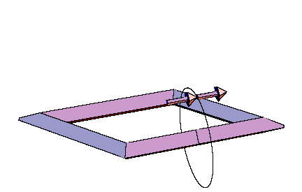
From the following two animated illustrations, which had been prepared with the kind help of Dr. E. Tjaden, we hope that you can get an imagination of these constructions.

Conclusion: The preceding considerations show, that a rather general concept of symmetry for curves in the plane and in 3-space leads to interesting versions of visible symmetries for them. These symmetries motivate in many cases why these curves are preferred for applications and for geometric constructions.